For HealthKPI‘s location features I need to deal with large(ish) quantities of spatio-temporal data. Basically, I have a bunch of time series with health data, and each data point has an attached location. Presently, I have around 10000 data points in my manually registered database, and I expect that number to only go up once I also allow automatically collected data. The question is now: how do I display this efficiently on a map?
Naturally, I cannot add 10000 data points to a map. That is just useless. Instead, I want some reasonable grouping, so all the datapoints gathered at my home is shown as a single (somewhat larger) point, as are datapoints gathered at other locations I frequent. If I zoom out on the map, I want all data points gathered in Eindhoven to be grouped, and if I zoom out further, I want data points to be grouped meaningfully for some value of meaningfully.
There are various clustering algorithms for such tasks, but they are all somewhat inefficient and none will really work well with 10000+ points on a mobile device in an interactive setting. Instead, I just build a simple index of all my data points.
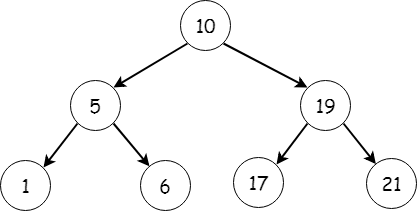
The index is really just an iteration of a binary tree. A binary tree stores elements on a number line so it is efficient to search for an individual item. It does this by defining a tree with a pivot element at the root and all values smaller than the pivot to the left and all elements larger to the right. To find a particular element, we just compare it with the pivot and either traverse the left or right depending on whether the element we look for is smaller or larger than the pivot. For example, if we search for 6, we can compare to the root, 10, and instantly avoid comparing the three elements to the right of the root as they are all larger than 10. If the tree is reasonably balanced, this means we can find elements in time that is proportional the the logarithm of the number of elements instead of linear. That means that in order to search 10000 data points, we only have to do 14 comparisons instead of 10000.
This works fine if you have data that can be ordered on a number line, such as numbers or strings (which famously obviously are numbers and therefore lice on a number line). Spatial coordinates cannot very meaningfully be ordered on a line, though, but they can easily be ordered on two lines, one for the latitude and one for the longitude. This gives rise to the quad tree: instead of only ordering elements based on a single value, we do it based on two values. Now a point cannot only be to the left or right of the pivot, but also above or below. This yields 4 (quad) directions Where a binary tree often only mentions the single pivot, a quad tree will typically mention both an upper and a lower bound. To search the quad tree, can rule out points in quadrants that do not contain our point similar to how we rules out values larger than 10 with a binary tree.
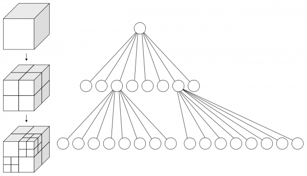
Taking spatial coordinates to a two-dimensional quad tree, the next step, moving to three dimensions is obvious. Normally, three dimensional octrees are used in 3D graphics. They exactly extend the 2D space with a third dimension, subdividing 3D space into 8 (octo) chunks instead of just 4 (quad). There is of course nothing preventing us from instead using the third dimension for time, leading to an octree with two spatial dimensions, latitude and longitude, and on temporal dimension, time.
Such a tree allows us to efficiently search for data points, no matter where they hide in the space-time continuum, as long as it is not moving above or below the Earth’s surface, which is frankly both preposterous and unnatural, but searching for points in time on a flat Earth was not really our goal. Our goal was to display a meaningful aggregate for a region if necessary. A plain quad or octree will not really help there, and especially not with our kind of data. The data in HealthKPI is very likely to be clustered around just a few data points: at home, at the pub, and and the liquor store. Remember when we discussed binary trees, I mentioned that the tree would have to be “reasonably balanced” for search to be efficient? Unless we do weird stuff, these trees are only going to be fair and balanced in the same sense that Fox News is.
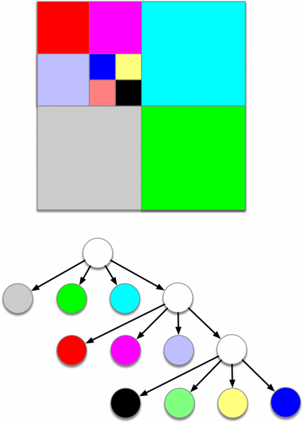
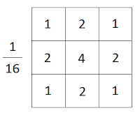
But that is ok. We are not interested in the nitty gritty details if there are a lot of points in a single location; that was actually the entire point: if there are 3000 data points at home, 3000 at the pub and 3000 at the liquor store, we want to treat them as just 3 points, and the quad tree structure actually helps us with that. Instead of searching to the leaf nodes at the bottom of trees, we just search to a level where we have sufficient detail. In the quad tree example above, maybe we have a meaningful level of detail for our map zoom level as soon as we enter the level of the red/magenta/lavender quads. Now, if the white node above the black, green, yellow and blue nodes contain sufficient information about them we do not have to look at them at all. Then, even if our octree is not balanced, it does not matter: we simply search until we reach the level of detail we need.
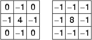
To figure out what we need to store in the white node to meaningfully aggregate the four nodes below, we look to image processing. Often, image processing needs to know the value of a number of surrounding pixels. This is for example the case when doing edge detection or simple blur using simple convolution filtering. Ignoring decomposition, this would entail adding 9 pixels for each pixels for a 3*3 kernel or 25 pixels for a 5*5 kernel. This is obviously very inefficient, especially with higher resolution images where we sometimes want to use a much larger kernel.
To get around this, image processing often computes the integral frame (shut up about linear decomposition of convolution filters). It just contains the sum of all pixels above and to the left of itself. That makes it possible to compute the sum of any area as a simple sum of 4 values, regardless of how large a kernel we wish to compute. The reason we compute the sum instead of some average is that using the sum we can compute the average afterwards, and we can then use a single integral frame to compute any average (so, we can comnpute the above blur by taking a 3*3 sum, adding the pixels above/below and to the left/right, and 3 times the central pixels, diving the whole thing by 16, or we can do the convolution for an edge detection by computing the 3*3 kernel and subtracting it from 9 times the central pixel.
We can do something similar for our octree. Now, we let all the central nodes contain the sum of the latitudes of all children, the sum of all longitudes, the sum of all registrations of all children, etc. If we also keep track of how many children a node aggregates, we can compute a meaningful average for all children contained in a node by taking the sum and diving by the number of children. Again, the reason for storing the sum instead of pre-computed averages is that it allows us to easily compute averages for other areas and to easily add new points to the tree without having to do massive recomputations. To add a new point below a node, simple add its latitude/longitude/registration to all parent nodes and increase the count by 1. This is much simpler and more numerically stable than operating with pre-computed averages.
Storing sums also makes it easy to compute values for areas that doesn’t exactly line up with the octree boundaries: given a bounding box, simply process nodes depending on which partition it falls into: Entirely contained: just use the sums stored in the node. Entirely outside: ignore entirely. Overlapping: recursively process all children. Since we are dealing with sums, we can simply add them up in any order without having to worry about weighing averages.
Now the clustering is simply: partition the viewed map area into, say, 10 blocks horizontally and 10 blocks vertically. For each of these 10*10 blocks, compute sums of latitude/longitude/registration and divide by the number of registrations for the area. Each of these computations become relatively simple as most of them will have no registrations at any level of zoom.
The temporal dimension is not optimal, because it is not obvious what the best time scale to location scale is, and most registrations are likely very localised spatially while spread out temporally (like 5 years of data at home) or vice versa (visiting 10 countries for 1-2 weeks at a time over a 5 year period). That does not mean it is useless, though. By storing time intervals in out aggregations, we can also use this index to filter out that one registration we made while nearly passed out drunk over the Atlantic (since we know the counts) or the 30 registrations we made in China 5 years ago. That way, the index also allows us to suggest a meaningful initial view of the map: search to the most specific node containing more than a lower threshold of registrations made within a given time period from now.
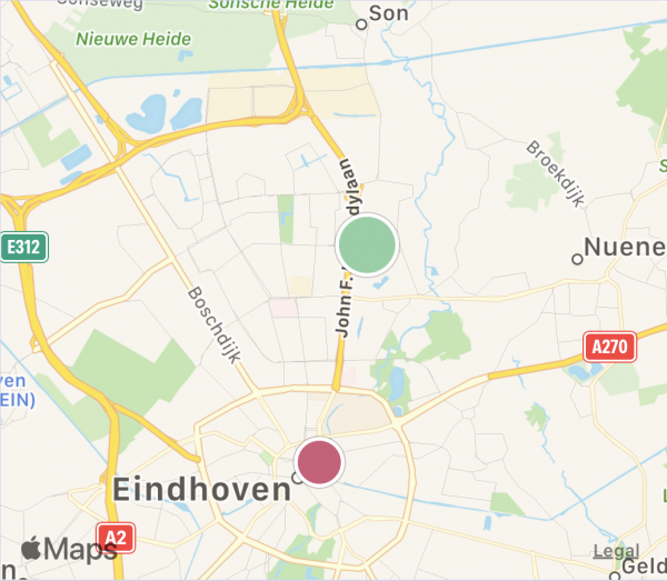
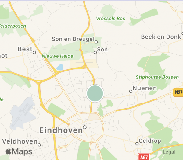
Combining all of this, we get to draw pretty maps like this. The first one shows the auto-zoom feature. Here, green represents positive values and red negative values. The size reflects how many data points each cluster represents. The second image zooms out a bit, thereby merging the two visible clusters (note that while at first sight, it looks like the red cluster just disappeared, really the green moved down slightly to reflect the new combined cluster center and the color went ever so slightly paler, to reflect the slightly lower average due to the red dot being merged in). The final map is just further zooming out.

None of this is of course terribly surprising or revolutionary, but it was still quite fun trying to implement. One of the biggest challenges was making Swift and CoreData cooperate with what I wanted (CoreData is an object persistence framework and not really suitable for even marginally fancy data structures that are not just simple object graphs). Trying to write the user interface using SwiftUI also proved challenging, because the MapKit APIs still are based on the older UIKit and a large chunk of ObjectiveC. While I have not given the code a test-drive with thousands or hundreds of thousands of points, I have a good feeling about the potential and will give it a whirl later (I am working on augmenting existing data with locations based on other available data to get more and realistic location data). As a bonus, here’s the map in (silky-smooth) action:
By the way, there is a “Where in Spacetime is Carmen Sandiego,” it’s just called Where in Time is Carmen Sandiego.