It’s been a while since I last wrote about the Model-based Testing Workbench. That’s not for lack of developments, but because I bit over what turned out to be much more complex and useful than I originally anticipated. That’s not the topic of this post, though, in this post I’ll outline a bunch of minor improvements that just make the tool nicer and more efficient to use.
If you recall, the MBT Workbench is a tool for supporting the model-based testing approach. We test web-services by generating requests from a set of input variables and extract output variables from the responses. We compare the output variables to a parallel derivation of the values from an abstract but formal and executable description denoted a model. The MBT Workbench assists the user in all the steps needed to achieve this. Last time, we took a look at how we generate a decision tree model automatically from a web-service. Prior to that, we took a look at how we semi-automatically can generate an input mapping from a WSDL.
In this post, we revisit first the input generation and then how models are displayed. The goal is the models should be as simple and powerful as possible, but most importantly be understandable. The models serve primarily to gain trust of the operation of the system since the correctness of operation and the generation of test cases is entirely based on them, so understandability is very important.
We shall continue using the same running example we have used so far: an insurance company grants car insurance to customers, but due to increased risk, insurance is not granted to males younger than 25. We have a web-service taking the age and gender of the customer and returning either an offer or a rejection.
Improved Input Mapping
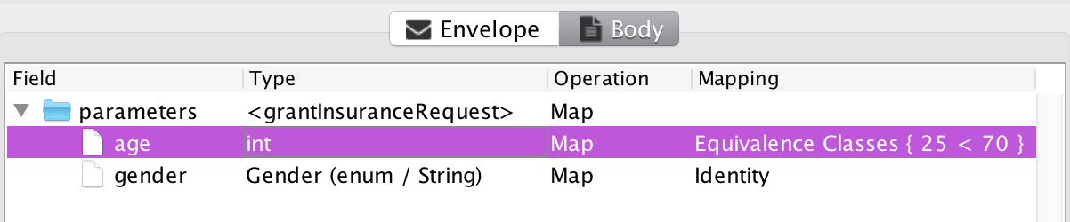
We set up the translation from the logical domain of ages and genders to the web-service in the MBT workbench like this (we assume that for some reason we believe that the age 70 also matters while setting up the test):
Previously, this would have resulted in a mapping like this:
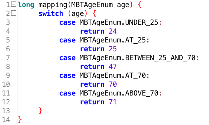
This is largely ok. We test the two interesting values, 25 and 70. We also test values surrounding the interesting the values, one value between the two interesting values, and two one the outside of the interesting values.
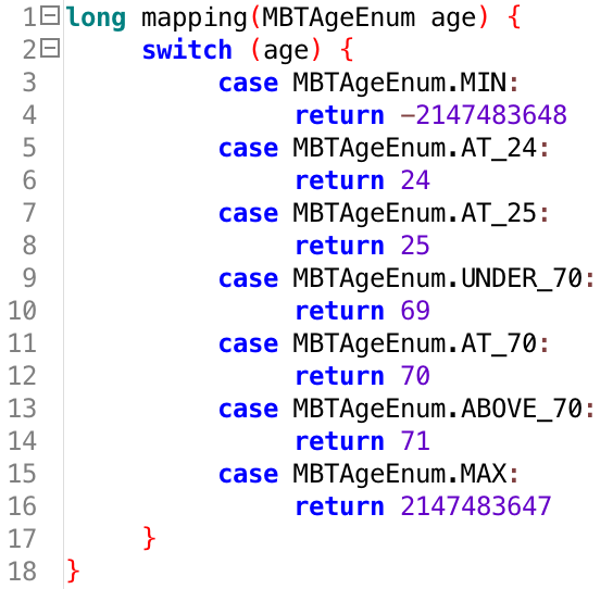
This specification does have some issues, though. Would a test catch if the implementation instead implemented the rule as “young men below 30 cannot get insurance,” for example? And how does it handle extreme values like 5000 years or outrageous values like -15 years? The mapping doesn’t really capture the full behavior of the system. For this reason, the mapping generation has been tweaked a bit, and now we instead emit:
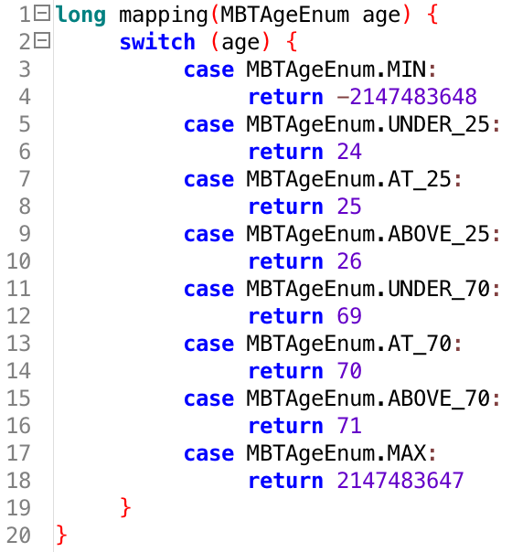
Now, we explicitly check that “largest possible” and “smallest possible” values. These values are determined based on the specified data type and limits in the WSDL. Here, we are using a signed integer and specify no limits in the WSDL, so in principle we go from -231 to 231-1 and the test reflects that.
We have also done away with testing the “between” values, and instead thoroughly test the interesting borders. If an implementation got the border slightly wrong, the test captures it.
This does increase the testing complexity some (we go from 2 * n + 1 to 3 * n + 2 test cases, where n is the number of interesting borders). To alleviate this some, I have also improved the syntax slightly, so we can now also use, say, 24/25, to indicate that the border 24/25 is interesting. The tool will then fit the limit more accurately instead of generating entries for both above and below the interesting limit. For example, if we specify our test like this:

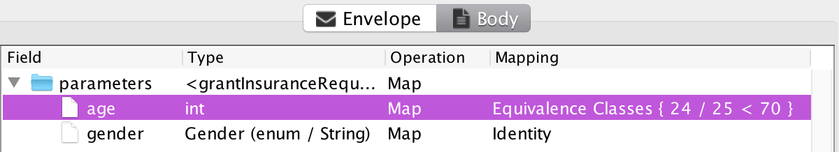
We get a mapping reflecting this extra knowledge:
Were we to also specify the border at 70 more precisely, we would go from 5 tested values to 6, in my opinion an acceptable increase for the increased quality and precision of the test. In my next post, I’ll detail a new function of the tool which will additionally help the user with this.
Improved Model Mining and Variable Set Display
Using the old mapping, we would obtain a model looking like this:
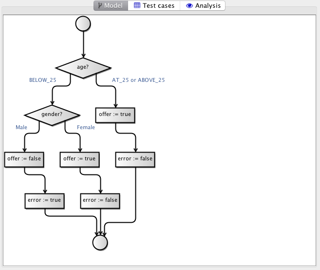
What the example doesn’t show is that for the new style mapping, we would instead have obtained multiple age nodes – the old model mining algorithm would only allow a choice node to split off a single value (BELOW_25 in the example). With the new mapping, we actually need to split off two values, MIN and AT_24, and the old way the old algorithm could cope would be to first split off the one and then the other. (Actually, this would in turn cause the algorithm to decide that first splitting up by gender is more beneficial.) This does not lead to a more understandable model.
In addition, we see that all possible values are listed on the alternative branch (AT_25 or ABOVE_25). This is manageable with few values, but less when the choices become more involved. For example, the BELOW_25 branch would become MIN or AT_24, which is not very readable (though more readable than the other branch which would become “AT_25, BELOW_70, AT_70, ABOVE_70, or MAX”) but also doesn’t reflect the logical case we try to capture very nicely.
To efficiently solve these issues, we now distinguish between “random” values and ordered values. Ordered values are directly totally ordered sets from algebra (though we are very lax on the anti-symmetry requirement). That just means that we can always decide which of two values are larger. For the example, it is easy to see that MIN ≤ AT_24 ≤ AT_25 ≤ UNDER_70 ≤ AT_70 ≤ ABOVE_70 ≤ MAX (because they directly map to real values).
To solve the first issue, the mining algorithm now supports mining subsets of values. This is in principle easy: just iterate over all subsets of the co-domain of each input variable when partitioning. The issue is that “all subsets” is exponential in size of the input, which in theory and in some practical example I experimented with has real impact – just going to 10 possible values, means we have to try 29 = 512 combinations (we only need to try half of the 210 combinations), and going to 20 would mean going thru 219 = 524.288 possibilities.
By exploiting the ordering property, we can meaningfully assume that we only need to try “connected” sets. I further add the restriction that sets should always contain the minimum value; that means we have to try sets like { MIN, AT_24 } and { MIN, AT_25, AT_25, UNDER_70 } but not sets { AT_25, AT_25 } (MIN is missing) or { MIN, AT_24, UNDER_70 } (AT_25 is missing to make the set connected). This reduces the options for the example to 6 options, or 9 for when we have 10 options or 19 when we have 20. This actually reduces the number of options tried by one compared to earlier (except for the case with exactly 2 values, where the tool was smart enough not to try both options).
We can use that same property to more efficiently display variable sets. We can just reduce such sets to the largest/smallest value plus “or less” or “or more.” Putting this together, means the model now starts like this:
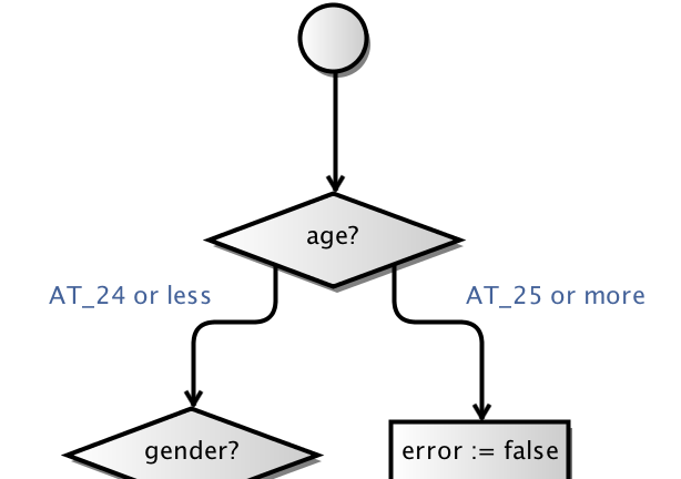
We don’t have to bother with the fact that we also include the artificial values MIN and MAX, nor do we even see the here uninteresting border around 70.
Improved Model Display
The original model at the top is decently understandable, but even for this simple case, we notice there is a lot of redundancy and the model doesn’t clearly reflect the cases that are the same and those that are different. To improve this, I made two improved models views which focus on each of these aspects.
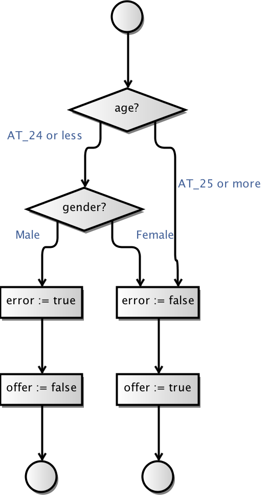
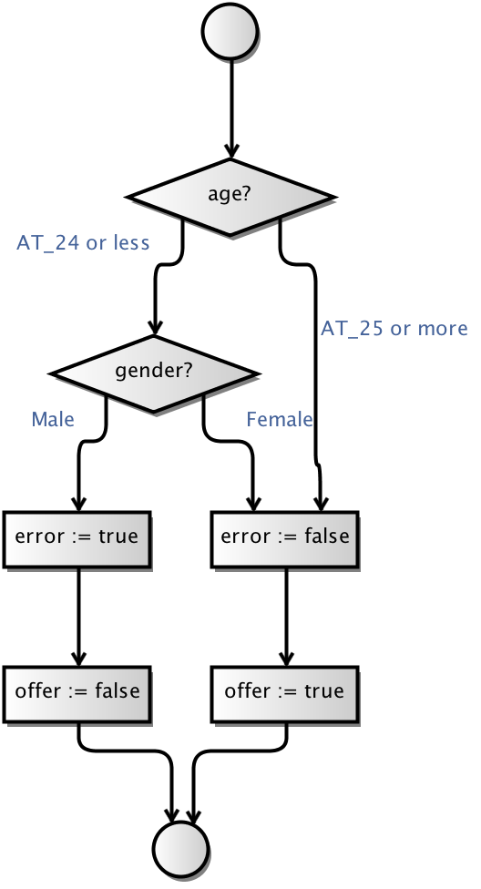
The first view aims to represent the end state explicitly. In the example, we have two end states: “got an offer” and “got a rejection.” To illustrate this, we duplicate the end node, and instead display the model like this:

It is now clear that the “AT_25 or more” branch merges with the “Female” branch to yield an offer, and the “AT_24 or less, Male” branch is different.
We still see quite a measure of redundancy in the model, though: the two “offer” branches contain a lot of identical nodes (well, two pairs of two). To improve on this, we also perform suffix tree reduction, where we merge identical suffix trees, leading to a cleaner result:
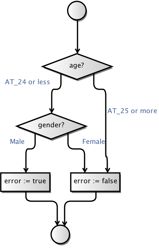
If desired, we can also use just the suffix merging without the indication of end-states. This can sometimes lead to a cleaner result:
These are of course all just display options, and really shine when used with the model optimization I explained in my previous post:
This is of course just a toy example, but for a model generated completely automatically, the result is very good in my opinion.
In this post, I have introduced 3 (4) minor improvements that make models more understandable. Next time, we’ll look at how the tool can help making the models better reflect reality by testing some of the (very few) inputs from the user for correctness.