The MBT Workbench, my tool for model-based testing, is nearing completion, at least in a proof-of-concept state. The idea is that instead of focusing on setting up test logical cases and manually or semi-automatically validating that an application adheres to them, we just provide a model describing the correct system behavior, and let the computer sort out what to test.
So far, we have been concerned with a bunch of technical things, most importantly mapping between the real-world and the model domain. We do this using input mappings and output mappings. Input mapping map the model domain to the real-world and the output mappings map real-world data back to the modeling domain. This way we can execute the model and real service in parallel check that the result is as expected.
The MBT Workbench provides tools to help users setting up these mappings. Input mappings are created by inspecting the service under test and asking the user to pick what is important and important boundaries for data (for example, an insurance company might treat customers differently based on age). Output mappings are pretty much the same.
Where things get really interesting is when it comes to the model part of the equation. The MBT Workbench is based on a meta-model of the testing process. This meta-model is reflected in the below GUI, and fundamentally allows users to set up the 3 essential artifacts (input mappings, output mappings, and models, not counting the system under test) in any order. Depending on the artifacts available, the tool can provide more help.
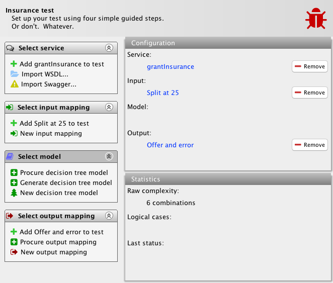
In the example, we have set up the input and output mapping. We have done this as explained in previous posts (input mapping, output mapping). The system under test is the example we have been using in all these posts: an insurance company is granting car insurances. Offers are made to customers based on age and gender. No offers are made to males below the age of 25. The input mapping is set up to try all possible values for ages (below 25, 25 exactly, and above 25) and genders (male and female). The output mapping detects whether an offer is made and whether an error is returned. This yields 6 combinations as shown.
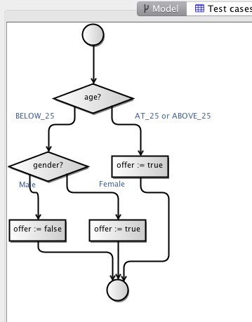
Now, finally, let us generate a model. This is done completely automatically. The tool invokes the service (stub really) to gather matching input and output values. It then constructs a decision tree based on these, end presents it as a flow-chart:
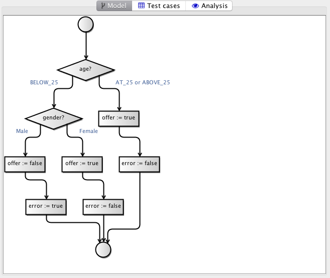
We can inspect this model and get a pretty good idea of what the system does: we first check the age of the applicant. If the age is 25 or above, we return an offer and no error. Otherwise, we check the gender and if it’s a young man, we do not return an offer but instead an error. If it’s a young woman, we return an offer just like for adults.
This model is generated entirely automatically, using a simple learning algorithm. The algorithm tries to identify which input parameter best separates the output. It does using a concept from information theory called the entropy. It is a measurement of randomness in data. The more random data looks, the higher the entropy. Data which consists on one value only has the lowest entropy. If we split by age 25, we get one partition, where everybody gets insurance and one where some do. In the case where everybody gets insurance, the entropy is zero (the result is the same for everybody), so age is a good splitter. We repeat the process until we have separated all data into partitions with entropy zero.
This results in a model in a simple DSL, which consists of choices and assignments. We render this language as a flow-chart as it is intended to be easily understandable as well as executable. The flow-chart is displayed using the JGraphX library (the Java equivalent and predecessor of the library used by draw.io).
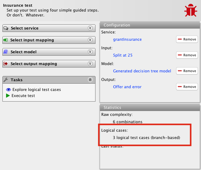
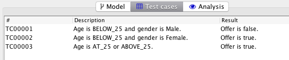
The advantage of this super-simple language is that it is easy to make quite sophisticated analysis. For example, we can infer the number of logical test cases. To do that, we turn to the notion of branch coverage from standard testing practices. The number of test cases assuming we go for 100% branch coverage is simply the number of arrows leading into the end node – the bottom circle – or, equivalently, the number of branching nodes – diamond nodes – plus one. It’s three in our example. As a matter of fact, once we add the model to our test, the tool shows this:
The tool can even infer descriptions of these test cases and the expected outcomes:
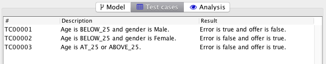
We note that for TC00003 the gender is not included in the description. That is because this is a case, much like love, where gender doesn’t matter: insurance is granted to everybody regardless of gender when they are above 25.
In my original post, I was dealing with 3 other logical test cases (male below 25, female, and male above 25). That is because I mentally had ordered the two decisions of the model differently, so I would branch on gender before age. This is functionally equivalent and coincidentally leads to the same number of logical test cases. There is no guarantee this is the case, though, so the MBT Workbench also allows users to optimize their models. Optimizing the generated model above, yields this model:
We notice that the error has been eliminated from both model and test cases. The tool has realized that the fact that an error is returned can be derived from whether an offer is returned (an error is returned if and only if an offer is not). Eliminating the variable simplifies both model and test cases. Remember, the test cases are only here for readability; the tool still does comprehensive testing of all possibilities. The logical test cases are only for documentation, so simplicity and understandability are important.
The optimization process works on any model regardless of how it was constructed. This means that once I add manual or semi-automatic model construction to the tool, the process can optimize the design automatically. This is for example useful for constructing a design based on the specification and running the tool to simplify the specification is applicable, and thereafter generate test cases based on the simplified design.
Consider if I had included the show size in the original model. It would add absolutely nothing to the system as it doesn’t matter to the decision process, but it would contribute to complicating the model, and would also contribute additional logical test cases. By optimizing the irrelevant variable away, we simplify the model and the test cases. If it is considered important for the actual testing, nothing prevents a user from still trying different shoe sizes – it will just not be reflected in the high-level summary.
The variable optimization is performed in two steps: first we eliminate redundant output variables, and then we eliminate redundant input variables and test cases.
Eliminating output variables is done by computing sets of variables that allow us to predict any other variable. Consider the below tables of values:
| a | b | c |
|---|---|---|
| 0 | 0 | 0 |
| 0 | 1 | 1 |
| 1 | 0 | 2 |
| 1 | 1 | 3 |
If we know the value of c, we can also predict the value of a. For example, if c is 2, we can just look in the row of c = 2 and see that a = 1. We can therefore eliminate a from the model. If we ever need it, we can just replace it by the “computation” we just performed.
We cannot predict the value of a from b. If b = 0, a can be both 0 or 1 (corresponding to c = 0 or 2). Similarly, we cannot predict b from a or c from either a or b. We can predict b from c like before, so it can be eliminated as well, leaving us with a model comprising c only.
In the same manner, we eliminated error from the insurance mode, as it could predicted completely from the offer.
Sometimes the situation is a bit more complex; consider this table:
| d | e | f |
|---|---|---|
| 0 | 0 | 0 |
| 0 | 1 | 1 |
| 1 | 0 | 1 |
| 1 | 1 | 1 |
It seems like we cannot predict any column from another (if d = 0, e and f can be either 0 or 1, if e = 0, d and f can be either 0 or 1, and if f = 1, d and e can be either 0 or 1). We can, however, predict the value of f from the combined values of d and e. If d = 0 and e = 1, we know that f = 1. Mathematically, this is the boolean operation or, but we don’t really care. We just know there is an operation that allows us to uniquely compute f from d and e in our single case, so we can eliminate f from the model, and get a simpler model comprising d and e only.
We perform this elimination until no more variables can be eliminated. At this point, we generate a decision tree based on possible input/output combinations. Remember that the starting model can be a decision tree or whichever other modeling language is supported (actually, we can consider the original model generation as a similar optimization where we use the real system as the model). The generation process is set up so it only considers variables necessary to partition the output variables fully.
This process will lead to a model with at most as many input and output variables as the input. Furthermore, the result will always be a decision tree model, regardless of which formalism was used as input, so whichever analysis techniques are implemented, they only need to be implemented for this one language. One example of such analysis technique is the test case generation, which relies on the structure of the decision tree.
We are nearing the end of this series – at least so far as I have planned. I have two posts planned out, and after that, I want to do some of the boring things I have postponed: environment management, handling more complex request, including requests with lists and requests with arbitrary contents, improved mapping editing, more pre-defined mappings, etc.
The two posts I have planned are: one where I finally tie it all together and perform a system test and generate a test report. Performing the test will be the easy part as I have all the components in place for this already. Setting up the reports will probably be done using JasperReports. The other planned post is less of a wordy ready one, and more of a planned video demonstration of the entire tool using the same case we have gone thru piecemeal in these posts.